Documentation for the Krigifier, Kriging Approximation, and Radial Basis Function
Approximation C++ Classes
Anthony Padula
This chapter will describe the quick and hopefully easy way to get
these classes running on your system. If you have difficulty with
these instructions, we refer you to Chapter 2 for
suggestions on things to try. The scripts and makefiles are designed
for Linux machines running g++ and g77. Users of other systems should
see Chapter 2 for suggestions on modifying the
provided files.
All the necessary software is available at
http://www.cs.wm.edu/~va/software. Follow the link to the
``Krigifier Classes'' which should be near the bottom of the page.
This will take you to the page where the krigifier and related
software is kept. Then you need to download three files
krig.tgz, netlibfiles.tgz, and installkrig. Hold down
the ``shift'' key and click on the links to these files in the
Compressed files section of the web page. Then save the files
to the appropriate directory.
If you already have gnu zip on your system, then you are ready
to install. Otherwise, click on the link to gnu zip and
download and install it on your system.
Once you have obtained the software, go to the directory where you
saved the files. Then, at your command line, execute the commands:
- chmod 700 installkrig
- ./installkrig
After the script finishes, the files have been unpacked and the
libraries have been built. To save some disk space, we suggest
deleting the directories clapack, blas, and libf2c.
The files in these directories have been stored in the archives
liblapack.a, libblas.a, and libf2c.a, so you don't need
the originals anymore. Type:
- rm -rf clapack
- rm -rf blas
- rm -rf libf2c
Be very careful to type these exactly.
A number of demo programs have been provided. Efforts have been made
to comment the code clearly so users can follow the executions.
To compile the demos all at once, type
make demos
This will handle all the compilation. To run one of the demos,
for example demo2, type
./demo2
Note that the demos may take some time to run. Be patient.
Several of the demos require an input file named krig.dat. An
example of this has been provided for you. This file is all of the
input. We have provided several extra dat files named krig.dat.new?.
Try copying these into krig.dat and rerunning the demo to examine
the different results. See section 3.9 for more
discussion of the various parameters. We also point you
to [2] (particularly Appendix B and Chapter 3) for further discussion.
The demos produce output into a file named results?.out.
Thus, demo2 outputs to results2.out.
The output file is a list of points in three dimensional space. These points are
evaluations of a function on a grid. If you have gnuplot, a
driver program has been provided to create postscript plots of the
demo output. For example, to graph results2.out, type
./plotpoints results2.out results2.ps
The driver will prompt the user for a title to add to the plot. Type
in the desired title and then press ``enter''.
This driver generates the file results?.ps, which contains a
plot of the points in theresults?.out file. To view these plots
using ghostview, type
gv results2.ps &
This starts ghostview running in a separate window. Alternatively,
you may print these plots by typing
lpr results2.ps
Several demo programs have been provided. They are very similar.
Each shows the use of slightly different options or different
classes. The classes are designed as much as possible with a
consistent interface.
It creates a random function, using the parameters specified in "krig.dat",
evaluates it at several sites, and uses these values to
create an approximation. The approximation is then evaluated systematically and the results
are output to the file "results.out"
We instruct the krigifier to do Latin Hypercube sampling.
It creates a random function, using the parameters specified on the function call.
It chooses to use a user-defined trend, described in TrendFunction(). It then
evaluates the function at several sites, and uses these values to
create an approximation, using the Gaussian isotropic correlation function
and passing in the known value of theta.
The approximation is then evaluated systematically and the results are output to the file
``results2.out'' while simple statistics on the data are output to the screen
Differences from ``demo1.cc'':
- krigifier parameters passed through function call, rather than being read from a file
- krigifier given specific rng seed and stream to use
- krigifier uses user-defined trend
- approximation given theta, instead of doing estimation
- calls analyzevalues() instead of scanfunction() in order to get more information
- Latin Hypercubes are used instead of Uniform Random sampling in the krigifier
This is an extremely simplistic demo. It creates an randfunc object,
randomly generates the function using parameter values from ``krig.dat'',
and then evaluates the function at a number of sites, outputing the results
to ``results3.out''.
It creates a random function, using the parameters specified in ``krig.dat'',
evaluates it at several sites, and uses these values to
create an approximation. The approximation is then evaluated systematically and the results
are output to the file ``results4.out''
This demo is very similar to the one in demo1.cc, except that
demo4 also evaluates the
derivatives of the kriging approximation instead of the approximation function itself.
The program keeps track of the point with the smallest function value
that it finds and displays this location
along with the derivative at this location.
It creates a random function, using the parameters specified in ``krig.dat'',
evaluates it at several sites, and uses these values to
create an approximation. The approximation is then evaluated systematically and the results
are output to the file ``results5.out''
This is indentical to demo1.cc except that it uses the krigapproxWithGLS class that has the
extra quadratic trend, as described in Section 3.5.1.
This is an extremely simplistic demo, much like demo3 It estimates the quadratic function
using the glsapprox class, as described in Section 3.5.1.
It then evaluates the estimate at a number of sites, outputing the results
to "results6.out"
If you have the wish interpreter (version 8.0, or else some other tk/tcl interpreter)
on your system, you can use the graphical interface provided to run
the krigifier. To do this type
- make kriggui
- ./kriggui
You will be presented with a window full of sliders. Move the sliders
to set the desired parameters, and then push the Plot button.
The program will then generate a function. When it is done
generating, it will beep and display a message stating that it is
finished. A gv window will automatically be opened and a graph
of the function displayed. You may then change the parameter settings
, reset the seed to -1, and hit Plot again to generate a new function. When the new
function has been generated, push the redisplay button beside
the plot in ghostview, in order to view the new plot.
If you get an error like
execve viewer: No such file or directory
you will need to go into the kriggui.cc file and modify the line
// The full pathname of your postscript viewer
char viewer[20] = "/usr/bin/X11/gv";
Change the ``/usr/bin/X11/gv'' to be the pathname for your
postscript viewer. It is likely stored in /usr/bin,
/usr/local/bin, /bin, or some such directory. Further, we have
a kill(gvid,SIGHUP); command in our code to tell gv to
update
the picture from the file. You should change the flag at the top of
the file to be bool redisplay = false and then push the equivalent of the redisplay
button on your viewer.
Currently, the program creates several temporary files. It creates
``kriggui.out'' and ``kriggui.ps''. If you don't want to keep the
last picture you created, be sure to delete these files later. If you
would like to save a picture, we suggest copying the ``kriggui.ps''
file to another name so that it doesn't get overwritten.
A number of features have been provided for your convenience.
The File menu at the top of the window has several useful
commands. You may exit the program by choosing Exit at the
bottom of the menu. The button labeled Sound at the top of the
menu toggles the beeps on and off. Then, you may Save and
Load parameter settings from text files. Notice that the format of
these files differ from that in the .dat files, like
``krig.dat'' mentioned earlier. Thus, do not try to
interchange these files. The order of inputs in the GUI data files
is:
- p
- n
- tau2
- beta0
- alpha
- theta
- sigma2
- lower
- upper
- seed
- stream
An example, using the default settings of the gui, is contained in the
file ``gui.dat''.
There is now a feature to convert between the two
styles of data files. These functions can be accessed from the
File menu. At the first prompt, enter the name of the file in which the data
is currently. Then, at the second prompt, enter the name of the
file to which to write. Each time, hit OK when you are finished
entering the file name. To quit conversion, hit Cancel. For
more help with converting files, please see the run-time Help menu.
Initially, the seed displayed is -1. This causes the program to
take a seed from the system clock and use it to generate a function.
This seed is then displayed for your benefit so that you may later
reproduce functions if desired. In the beginning, we recommend you
type -1 in the seed box each time, so that the program will continue
to take seeds from the system clock. However, should you find a
function you would like to be able to reproduce, be sure to note the
seed and stream. If you later want to generate the same function, you
must set the parameters to the same value and type the appropriate
seed and stream into the boxes. For example, we are quite fond of the
function given in the ``gui.dat'' file. You may load this file using
the Load feature. Notice how the seed 962042702 and stream
42 are displayed in the boxes. Were these changed, a different
function would be produced.
2. Troubleshooting
If you have difficulty in installing or executing the code, there are
several things which may be wrong. We have suggestions that may help
the problem.
Sometimes the provided script will not work completely. In these
cases, the last thing displayed should be some sort of manual page or
command options list. In this section we give several suggestions for fixing this
problem.
The files provided have been run through gunzip and tar to
compress them. You can unpack these files by typing
- gtar zxvf krig.tgz
- gtar zxvf netlibfiles.tgz
If this fails, and it complains that it doesn't recognize the command
gtar, then try instead
- gunzip krig.tgz
- tar xvf krig.tar
- gunzip netlibfiles.tgz
- tar xvf netlibfiles.tar
If this still fails, you should obtain the unzipping programs from
http://www.gzip.org/, and then try again.
If you use a compiler other than gcc and g77, you will
need to modify both the installkrig script and the
Makefile. Open the script in a text editor, like emacs or vi, and
replace the references to gcc and g77 with ones to your C
and FORTRAN compiler. Then save and try running the script again. If
it still fails, you will also need to modify the makefile that is
provided along with libf2c. You can do this by changing to the
directory libf2c. There are several makefiles here, and a
README file. Read the README, select the appropriate makefile, and
modify it according to the instructions given.
One modification we have figured out is that on a Solaris system, you
need to change the line in makefile.u that reads
ld -r -x -o $*.xxx $*.o
to be instead
ld -r -o $*.xxx $*.o
This is described in the comments to the makefile.
If such modifications do not work, we suggest talking to your local systems adminstrator and
request that they install CLAPACK, BLAS, and/or F2C. You could also
ask that they get the free g++, gcc, and g77 from
the Free Software Foundation at http://www.gnu.org/.
If you have difficulties getting the demos to compile, there are a
couple things to try
If you use a C++ compiler other than g++, you will need to edit
the Makefile. This is easily done. Open the Makefile in
your text editor, and find the line that reads
CC=g++
Change the ``g++'' to be the name of your C++ compiler. You may also
need to change the line below that reads
CCFLAGS=-g -Wall -O
We have flags there for the debugger and optimization. We suggest
turning the default optimization on your compiler on with the
appropriate flag. If you don't
have a C++ compiler, obtain the g++ compiler from the Free
Software Foundation at http://www.gnu.org/.
Make is a standard UNIX utility for handling compilation efficiently.
If you do not have make you will have to do the compilation
manually. The simplest approach is to find the line in the
Makefile, and base your commands on that. For example, where the
Makefile says
demo1: krigify.o demo1.o rngs.o rvgs.o krig.o\
	gamma.o ParamEstimate.o DirectSearch.o\
	PatternSearch.o CompassSearch.o approx.o
	$(CC) $(CCFLAGS) demo1.o krig.o krigify.o rngs.o rvgs.o\
	gamma.o ParamEstimate.o PatternSearch.o CompassSearch.o\
	approx.o DirectSearch.o $(LIBS) -o demo1
you should type on the command line, all on one line
g++ -g -Wall -o demo1.cc krig.cc krigify.cc rngs.c rvgs.c gamma.cc
ParamEstimate.cc PatternSearch.cc CompassSearch.cc DirectSearch.cc
approx.cc -L./ -lLAPACK -lBLAS -lf2c -o demo1
Generally, fill in the macros with the given text at the top of the
file, i.e. replace $(CC) with g++. Then for most files replace the ``.o'' at the end with a
``.cc''. A few certain files get a ``.c'' instead. Look at the list
of files in your directory to determine which ones. Worst case, you
can just compile all of the ``.cc'' and ``.c'' files together
with one of the ``demo?.cc'' files.
If you have the compiler working, but it reports errors that it cannot
fix, then there is a little more difficulty in straightening thing
out. The first thing to do is to check to see if you are using the most
recent version of the compiler. If not, request that it be upgraded.
In particular, our implementation makes use of templates, which are a
newer feature.
We have noticed some portabilty difficulty with the new try/catch
style of memory allocation.
We are using g++ version 2.95.2. We have found that if you are
using an older version of the compiler, you may encounter errors
similar to
``try'' is a reserved word. Exception handling not enabled.
In this case, you will need to add the flag -DDOLD_ALLOC to the
compile command. The easiest way to do this is to edit the
Makefile and change the line
CCFLAGS=-g -Wall -O
to read instead
CCFLAGS=-g -Wall -O -DDOLD_ALLOC
If you still encounter difficulties, you should then also add the flag
-DOLD_LIBC, thus making the line in the Makefile read
CCFLAGS=-g -Wall -O -DDOLD_ALLOC -DOLD_LIBC
These flags have the same effect as putting a
#define DOLD_ALLOC
#define OLD_LIBC
in your code. They instruct our code to use the older libraries and
the old style dynamic allocation (= new then assert ) instead of the newer
try/catch.
If the compiler is up to date, then the problems are harder to fix.
At this point it becomes necessary to tinker with the code itself.
Often times there are slight differences in syntax or semantics
between compilers. Our code was written on a Linux system with Intel
Pentium II and III chips. We used the g++ compiler version 2.95.2.
The best suggestion we can offer is to find someone who is familiar
with cross-compiler difficulties who might recognize the problem.
We have tested all the code to some extent. However, we have not been
exhaustive. The code is fairly robust, and will warn you some if you give
it bad input. The demos are straightforward, and users are encouraged
to modify them to try out the advanced features described in the next
chapter.
If you see a message that
complains ``CHOLESKY : WARNING - A is not positive definite at row
72'' or something similar, it's okay. This is to be expected
sometimes. We have used the Cholesky decomposition in our
implementation, which requires the matrix to be positive definite.
Although the matrices are theoretically positive definite, they are
often not numerically positive definite. When the Cholesky
decomposition fails, this error message is printed. The program will
then try alternate methods which are slower, but will always work.
This is a feature, not a bug.
One other issue to be aware of - these algorithms can take a
significant period of time to run on large matrices. The complexity
is  where
where  is the number of interpolated points.
Extensive efforts have been made to do computations efficiently, but
the matrix factorizations in particular take a long time on large
matrices. You should use the optimization features of your compiler.
If this still takes too long, consider decreasing .
Occasionally, we've run into an error while using plotpoints.
The error reads something to the effect of
is the number of interpolated points.
Extensive efforts have been made to do computations efficiently, but
the matrix factorizations in particular take a long time on large
matrices. You should use the optimization features of your compiler.
If this still takes too long, consider decreasing .
Occasionally, we've run into an error while using plotpoints.
The error reads something to the effect of
Warning: Can not contour non-grid data
What this means is that the data in the file you gave as input to
plotpoints is bad. This ussually seems to be the result of either
running out of disk-quota or else it comes from terminating a program
early. You should check your disk space. If you need to free up
space, do so. Then execute the main program again to regenerate the
set of data. Then try plotpoints once more. If this still
fails, we suggest examining the data set, and trying to determine
where the error in the output lies.
Sometimes, you will get an error like
line 0: undefined variable: eps
This means that your version of gnuplot does not support encapsulated
postscript. Make certain you are not using the -e flag. If you
still have difficulties, you can always delete the word ``eps'' in the
one place in plotpoints.c that it appears. It's around line 69.
You may already have CLAPACK, the BLAS, or the f2c libraries installed
on your system. In this case, we recommend using the existing libraries
instead of the files we provided. You can place symbolic
links (using ln -s /wherever/your/files/are/kept/libfile.a
ourlibname.a) named appropriately (libLAPACK.a,
libBLAS.a, or libf2c.a) in your directory. Otherwise, you can
modify the Makefile by changing the LIBS macro to be
LIBS=-L/wherever/your/files/are/kept/ -lyourlibs
where your library files would be named libyourlibs.a in the
example given above.
NOTE:  THE FOLLOWING SECTIONS ARE INTENDED FOR ADVANCED USERS ONLY.
WE RECOMMEND EXPERIMENTING WITH THE BASIC PROGRAM BEFORE MOVING ON
TO THE ADVANCED OPTIONS.
Many of the advanced features are consistent between the
randfunc, krigapprox, and rbfapprox classes. Thus, we
will describe them by feature instead of by class, and make careful notes of
where the differences are.
These classes are written in C++, using the modified TNT libraries
Vector<>
and Matrix<> classes as modified by Chris
Siefert [3].
The krigifier can
generate a random function from one of several families of functions,
which can then be evaluated at one or more points in the space. The
idea for the krigifier is based on the underlying fiction of the
stochastic process used in kriging. By modeling this stochastic
process, we can create pseudo-random functions, which can then be used
as tests for algorithms. The algorithm for the krigifier is
described in Padula [2]. For more detail on the
mathematics behind the krigifier, we suggest referring to Trosset [4]
The kriging approximation works on a given set of initial locations and
functions values for those locations. The class creates an approximation,
which can then be evaluated at one or more points in the space. This class is designed to
behave much like the krigifier, except it is given the
data to interpolate instead of randomly generating it.
The krigapprox class is a direct implementation of the kriging methodology described in
Padula [2]. It estimates the needed parameters based on the data, then
constructs the correlation matrix  and calculates and stores the vector
 . Then, given a point at which to evaluate the approximation, it calculates the
vector
. Then, given a point at which to evaluate the approximation, it calculates the
vector  , multiplies by
  , and adds in the value of the trend. The trend is
estimated using linear least squares.
The radial basis function approximator takes input, similar to the
input given the kriging
approximation, builds the approximation based on the input, and can
then be evaluated at desired locations. The algorithm differs from
the kriging approximator, mainly in the type of basis functions.
Further, whereas the kriging estimates a covariance structure from the data,
the radial basis function msut be given the necessary parameters.
However, it is quite robust, and one set of parameters works fairly
well for many different data sets.
The method of using these classes is very similar. First you should
include the appropriate header file(s), for example, #include
"krigify.h". Then, in your code, there
are generally three steps:
, and adds in the value of the trend. The trend is
estimated using linear least squares.
The radial basis function approximator takes input, similar to the
input given the kriging
approximation, builds the approximation based on the input, and can
then be evaluated at desired locations. The algorithm differs from
the kriging approximator, mainly in the type of basis functions.
Further, whereas the kriging estimates a covariance structure from the data,
the radial basis function msut be given the necessary parameters.
However, it is quite robust, and one set of parameters works fairly
well for many different data sets.
The method of using these classes is very similar. First you should
include the appropriate header file(s), for example, #include
"krigify.h". Then, in your code, there
are generally three steps:
- Declare an instance of the class. This is done by a
statement like
randfunc MyRandomFunction;
This is just like declaring an integer. Your first put the type of
the object - in this case randfunc - and then put what you would
like to name the variable.
- Give the class input You should then run one of the
setvalues functions. Input can be read from the keyboard, a file, or
can be passed as parameters.
MyRandomFunction.setvalues();   // Read from keyboard
MyRBFApproximation.setvalues( "infile.dat" );  // Read from file
MyKrigingApproximation.setvalues(Points, Values, 1);  // Read from given parameters
- Evaluate the function You can then evaluate the function
by calling evalf().
y = MyRandomFunction.evalf(x);
Here,  is a Vector<double> as described in ``vec.h''. The
value
is a Vector<double> as described in ``vec.h''. The
value  returned is a double.
Notice that when reading in data from a file or the keyboard, vectors are input by
typing the values with spaces between them. For example,
 would be input as
Matrices are input by treating each row as a vector. For example,
we could enter an upper-triangular matrix as
or equivalently
All necessary files are currently stored on Virginia Torczon's web site,
http://www.cs.wm.edu/~va/software. They can be downloaded from there.
There are a number of shared files used by all three classes. They are:
- maps_general.h
- vec.h
- cmat.h
- Dyn_alloc.h
- gamma.h and gamma.cc
- approx.h and approx.cc
The krigifier requires several additional files
- krigify.h and krigify.cc
- rngs.h and rngs.c
- rvgs.h and rvgs.c
In addition to the shared files, the kriging approximation requires
- krig.h and krig.cc
- ParamEstimate.h and ParamEstimate.cc
- PatternSearch.h and PatternSearch.cc
- CompassSearch.h and CompassSearch.cc
- DirectSearch.h and DirectSearch.cc
- objective.h
Finally, the radial basis function approximation needs
You also need links to the necessary library files. The libraries used are the CLAPACK
and the BLAS. This also requires using the F2C libraries.
These classes all work off a choice of a basis function. In the
kriging, we call it a correlation function. In all of the classes,
users can select one of the built in basis functions, or they can
specify their own.
3.4.1 Optional Correlation Functions
In the randfunc and krigapprox classes, the member
function
chooseCorrelationFamily( int choice ) may be
called to choose among the hard wired correlation functions.
Currently, the options are:
- choice = 0
- User specified function (See below)
- choice = 1
- Gaussian isotropic

- choice = 2
- Gaussian product
- choice = 3
- Product of Linear
- choice = 5
- Matérn correlation function
where  is the degree
  modified Bessel function of the third order.
The default choice is Gaussian isotropic, so you really only need to run
this function in order to choose one of the other families.
Notice that choices 2 and 3 take a vector of theta and a single alpha,
while choice 5 takes a vector of theta and a vector
of alpha. Also, with choice 5, the alpha values MUST be all integers. Your input
when running setvalues() must be appropriate to the correlation function.
In the krigifier,
newrand() must be called after changing the
correlation function (note that the setvalues() function
calls newrand(). Otherwise, in both the krigifier and the
kriging approximation you should call
setvalues(). If you don't, your results will be nonsense.
We suggest that the order of function calls be, for example:
modified Bessel function of the third order.
The default choice is Gaussian isotropic, so you really only need to run
this function in order to choose one of the other families.
Notice that choices 2 and 3 take a vector of theta and a single alpha,
while choice 5 takes a vector of theta and a vector
of alpha. Also, with choice 5, the alpha values MUST be all integers. Your input
when running setvalues() must be appropriate to the correlation function.
In the krigifier,
newrand() must be called after changing the
correlation function (note that the setvalues() function
calls newrand(). Otherwise, in both the krigifier and the
kriging approximation you should call
setvalues(). If you don't, your results will be nonsense.
We suggest that the order of function calls be, for example:
randfunc TestFunction();
TestFunction.chooseCorrelationFamily( 2);
TestFunction.setvalues( filename );
TestFunction.evalf(x);
NOTE: IN THE KRIGING APPROXIMATION, PARAMETER ESTIMATION ONLY
WORKS ON THE GAUSSIAN
CORRELATION FUNCTIONS. This means you do not need to give the
correlation function parameters  and
and  for choices
1 and 2. Otherwise, the user must supply the
needed parameters when using the other correlation functions.
This is an alternative to the previous function. It allows the user to
pass in a correlation function of their own. The correlation
function must accept two equal length vectors as input and is expected to return a
double through the third output parameter.
This sets the choice to option 0, and choosing another choice later will
use a different correlation function without overwriting the
pointer. Thus, you may switch back and forth between a hard-wired function and a
user specified function by indicating a new choice as directed above.
An example of this would be the calls:
for choices
1 and 2. Otherwise, the user must supply the
needed parameters when using the other correlation functions.
This is an alternative to the previous function. It allows the user to
pass in a correlation function of their own. The correlation
function must accept two equal length vectors as input and is expected to return a
double through the third output parameter.
This sets the choice to option 0, and choosing another choice later will
use a different correlation function without overwriting the
pointer. Thus, you may switch back and forth between a hard-wired function and a
user specified function by indicating a new choice as directed above.
An example of this would be the calls:
randfunc TestFunction();
TestFunction.chooseCorrelationFamily( myCorrelationFunction );
TestFunction.setvalues( filename );
TestFunction.evalf(x);
You might define a correlation function as such:
 void myCorrelationFunction( const Vector<double>&,
                             const Vector<double>& y,
                             double & result  ){

 // Compute the correlation here

       result = computedCorrelation;
} // end myCorrelationFunction
The important, necessary features are accepting two equal length
vectors and returning a double via the parameter result. These are expected by the
randfunc class and it will not function properly otherwise.
NOTE: NOT EVERY ARITHMETIC FUNCTION WORKS AS A CORRELATION FUNCTION.
Correlation functions are expected to return values between
0 and 1. A value close to 1 indicates a strong
correlation, meaning that the function values at the two
points should be close
together. A value of 1 implies that the function values
should be identical. A value of 0 means that the function
values are completely unrelated.
A useful thing to note - the Vector<double> class has functions
dim() and size(), both of which return the size of the vector.
Thus, it is unnecessary to pass the size as a parameter of the
correlation function. Further, one may use either FORTRAN or C style array
referencing. See the file vec.h for more details.
Also, when using a user defined correlation function, the user is
responsible for storing the parameters of the function, as the
data members of the randfunc class are protected.
3.4.3 Optional Radial Basis Functions
Similarly, you can select among the radial basis functions provided
in the rbfapprox class.
The function chooseRBF(int choice, double c, double beta, long deg) allows the user
to pick a non-default basis function. The parameter choice specifies which
function. The default is choice = 7. The choices of functions are:
- 0
- User specified function (See below 3.4.4)
- 1
- Thin-plate splines:
 where
where  and
and  not even.
- 2
- Gaussian:
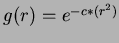 where
where  .
.
- 3
- Multiquadrics
 where
where  and not
even,
and not
even,  .
.
- 4
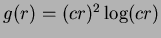
- Thin-plate splines
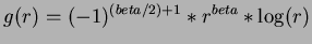 for
even.
for
even.
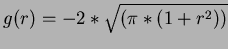
- 5
- Sobolew splines
 where
where
 ,
,  .
.
- 6
- Thin-plate splines
 . The literature suggests
  .
.
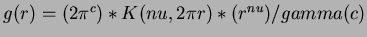
- 7
- Madych & Nelson II [1] pg 221
 .
.
where is the degree modified Bessel function of the third order.
This function automatically constructs the new approximation. setvalues() must have
been run prior to using chooseRBF().
3.4.4 User-Defined Basis Functions
You may use the function chooseRBF( void *RBFtoUse, long deg) to tell the
approximation to use some other basis function. The first parameter is the name of the
user-defined function. The second parameter is the degree as defined in
section 3.9.3. Such functions should take two parameters. The first is to
input the value
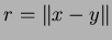 . The second is a reference parameter to return the
result. For example, the prototype for the user-defined function might be
. The second is a reference parameter to return the
result. For example, the prototype for the user-defined function might be
void myRBF(double /*input */ r, double\& /*output */ result);
and then the calling sequence could be
rbfapprox testrbf;
testrbf.setvalues(filename);
testrbf.chooseRBF( myRBF, deg);
This sets the choice to option 0, and choosing another choice later will
use a different correlation function without overwriting the pointer.
Thus, you may switch back and forth between a hard-wired function and a
user specified function by indicating a new choice as directed above.
NOTE: NOT EVERY ARITHMETIC FUNCTION WORKS AS A RADIAL BASIS FUNCTION
Be sure to choose deg appropriately for your function. If you are unsure,
use deg = p to be safe.
In the krigifier
the user may specify a non-quadratic trend through use of the setTrend()
function. The trend function requires two parameters, a const
Vector<double>& for input of the point at which the trend should
be evaluated, and a double & for returning the result. An example
of this would be:
void myTrend( const Vector<double>& x, double& result) {
     long p = x.size();

     result = 0;
     for(int i = 0; i<p; i++)
	     result = result+x[i];

     return;
} // end myTrend()
You can specify a trend like this:
randfunc TestFunction();
TestFunction.setTrend( myTrend );
TestFunction.setvalues( filename );
result = TestFunction.evalf( x);
This will replace the default quadratic trend. The setvalues()
functions will then no longer attempt to read in the parameters of the
quadratic trend. Thus, you cannot use the same data file for both
quadratic trended functions and functions with user-defined trends.
One new feature of the krigifier is the ability to randomly generate
quadratic trends. This is done by calling the function
TestFunction.generateTrend(tau2, &beta0);
This function should be called after calling the
setvalues function. It overwrites the read in quadratic trend with
a randomly generated one of the form
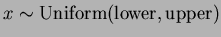
where  is chosen uniformly from the hypercube
![$[ lower +
(upper-lower)/4, upper - (upper-lower)/4 ]$](img40.png) and
and
 where the matrix
![$Y = [ y_{i,j} ] $](img42.png) is compsed of
is compsed of
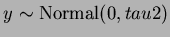 .
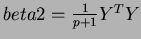
Generally, we can think of
.
Generally, we can think of  as specifying the height of the
minimum of the trend, and
as specifying the height of the
minimum of the trend, and  as the curvature of the quadratic
trend. Larger values of result in steeper trends.
When choosing a value for you will need to consider the current
values of
as the curvature of the quadratic
trend. Larger values of result in steeper trends.
When choosing a value for you will need to consider the current
values of  and the size of the space. The same will
produce very different looking results in different size spaces.
and the size of the space. The same will
produce very different looking results in different size spaces.
3.5.1 Kriging with Quadratic trends
As a new feature, there is a way for users to perform kriging and
estimate an underlying quadratic trend. Normally, the kriging works
with a constant trend. To do the quadratic trend instead, you will need the files
gls.h and gls.cc. Include gls.h in your source, and then
instead of declaring a krigapprox object as you would have done,
you should declare a krigapproxWithGLS object like this
krigapproxWithGLS MyKrigingApproximation;
After this, everything else works as normal.
By default, the krigifier uses uniform random sampling to generate the
set of initial design sites. We have also provided the option to use
other initial designs
3.6.1 Optional Initial Designs
The member function chooseInitialDesign( int choice ) may be
called to choose among the hard wired initial designs.
Currently, the options are:
- choice = 0
- User specified design (See below)
- choice = 1
- Uniform Random Sampling,
 .
.
- choice = 2
- Latin Hypercubes
The default choice is Uniform Random Sampling, so you really only need to run
this function in order to choose one of the other designs.
newrand() must be called after changing the initial design, either
directly or via setvalues(). Otherwise your results will be nonsense.
We suggest that the order of function calls be, for example:
randfunc TestFunction();
TestFunction.chooseInitialDesign( 2);
TestFunction.setvalues( filename );
TestFunction.evalf(x);
There is an alternative to the previous function.
This allows the user to specify an alternative initial design. The
initial design must accept four inputs:
- p
- the dimension of the space
- n
- the number of initial design sites (how many points in the space)
- lower
- the vector of lower bounds (rectangular spaces)
- upper
- the vector of upper bounds
The output parameter  is then the matrix in which the points
will be stored. is an
is then the matrix in which the points
will be stored. is an  matrix, with one point in each row.
This sets the choice to option 0, and choosing another choice later will
use a different correlation functiondesign without overwriting the
pointer. Thus, you may switch back and forth between a hard-wired designs and a
user specified design by indicating a new choice as directed above.
An example of this would be the calls:
matrix, with one point in each row.
This sets the choice to option 0, and choosing another choice later will
use a different correlation functiondesign without overwriting the
pointer. Thus, you may switch back and forth between a hard-wired designs and a
user specified design by indicating a new choice as directed above.
An example of this would be the calls:
randfunc TestFunction();
TestFunction.chooseInitialDesign( myInitialDesign );
TestFunction.setvalues( filename );
TestFunction.evalf(x);
You might define a design function as such:
 void myInitialDesign( const long p, const long n,
                       const Vector<double>& lower,
		       const Vector<double>& upper,
		       Matrix<double>& X) {

 // Compute the design matrix here

       X = theNewDesignMatrix;
} // end myInitialDesign
The important, necessary features are accepting two long
integers, and two equal length
vectors and returning a matrix of doubles via the parameter result. These are expected by the
randfunc class and it will not function properly otherwise.
There are a variety of accessor functions to retrieve the values of
some of the private data members of the various classes.
The ones available for all the classes are:
- long getp();
- long getn();
In the krigifier, there is also
- double getbeta0();
- Vector<double> getbeta1();
- Matrix<double> getbeta2();
- Vector<double> getx0();
- double getalpha();
- double gettheta();
- Matrix<double> getX();
- Vector<double> getv();
- Vector<double> getlower();
- Vector<double> getupper();
- long getSeed();
- int getStream();
The kriging approximation has
- Vector<double> getv();
- Vector<double> gettheta()
The RBF approximation has
- double getc()
- double getbeta()
Thus any of the initial inputs as well as some of the computed values can be retrieved.
I have included with the classes several non-member functions
that may be useful to a user. Notice that the rbf and kriging
approximation are derived classes, with the approx class as
a parent. Thus, wherever you see approx, it means you may
pass in either a krigapprox object or a rbfapprox object.
For the krigifier, we have
double reportsample(randfunc& Func, Vector<double> x, ostream& outf)
This function acts similarly to the member function evalf(). It
returns the value of the function at , and also makes an entry
in the output file. The function outputs the elements of x in
order of increasing dimension, ie.
![$x[0], x[1], \ldots, x[p]$](img50.png) , with a
blank space between each number. It then outputs the value of
the function at , followed by an end-line. Thus, the line in the
output file would look like:
, with a
blank space between each number. It then outputs the value of
the function at , followed by an end-line. Thus, the line in the
output file would look like:
if
 and
and  .
Similarly, for the approximations, we have
.
Similarly, for the approximations, we have
double reportsample( approx\& Func, Vector<double>\& x, ostream\& outf); }
This operates in exactly the same manner as the previous function.
We have a set of functions that output a sample of the given object at
a number of points. The differences between the krigifier versions and
the approximation versions is that the krigifier stores its own
bounds. Thus, in the approximation versions, there are two additional
parameters for passing in the lower and upper bound vectors.
void scanfunction(randfunc& Func, ostream& outf, int pointsperaxis)
void scanfunction( approx& Func, ostream& outf, long pointsperaxis,
                   Vector<double>& lower, Vector<double>& upper);
scanfunction() takes as input the object to be sampled
and an ofstream to output the values. It should work for any
value of p. It select pointsperaxis evenly spaced values on each axis, and
samples the function at every combination of values. The points
are spaced on a grid determined by the upper and lower bounds. The output
for each sampled point is done by reportsample(), and the format
of the output is the same as above, with one point to each
line. Output from scanfunction() is suitable for being
sent to gnuplot if  .
.
void scanfunction( randfunc& Func, ostream& outf);
void scanfunction( approx& Func, ostream& outf,
		   Vector<double>& lower, Vector<double>& upper);
This is simply a backwards compatible version that uses a default
25 points per axis.
void scanplane( randfunc& Func, ofstream& outf, int pointsperaxis);
void scanplane( approx& Func, ofstream& outf, int pointsperaxis,
  		Vector<double>& lower, Vector<double>& upper);
This is a slightly faster version of scanfunction() that ONLY
works on  functions. It outputs in a nice format for reading
or sending to gnuplot.
functions. It outputs in a nice format for reading
or sending to gnuplot.
void analyzevalues(randfunc& Func, ofstream& outf, int pointsperaxis);
void analyzevalues(  approx& Func, ofstream& outf, int pointsperaxis,
		     Vector<double>& lower, Vector<double>& upper);
Works much like scanfunction(), except that it reports simple statistics on
the points sampled to standard I/O, such as maximum value, minimum value,
average value, and the approximate location of the 25th and 75th
percentiles.
It divides each axis into pointsperaxis evenly spaced points, and samples at
each permutation of values.
Warning: This function stores all sampled points in memory. In higher
dimensions, this may fill up the available memory. Use at your
own risk. If you experience memory problems, try setting
pointsperaxis to a smaller value.
void analyzevalues( randfunc& Func, ofstream& outf);
void analyzevalues( approx  & Func, ofstream& outf,
		    Vector<double>& lower, Vector<double>& upper);
A default version that divides each axis into 25 evenly spaced points, and samples at
each permutation of values.
For the approximations, we have implemented a way to store their
values to a file in the same format it would have been read in. This
provides a method for storing approximations for later use.
void storeApprox( ostream\& outf );
This is a member function of the class, so you might call it as
MyKrigingApproximation.storeapprox(outf);
In the krigifier, there are two functions provided so that we may
reuse an object multiple times without re-inputting the
parameters. To get a new set of initial sites using the same parameters, one
may use the newrand() function:
TestFunction.newrand();
This generates a new and new . If you wish to use the same
initial sites but generate new values for them, ie keep and create
a new , use the newrandsameX() function instead. You may also call
setvalues() again and input a new set of parameters; The class
then generates new random components automatically.
3.9 Description of Parameters
For each of the classes there are a number of necessary parameters.
We describe them here for the benefit of new users. All
parameters are double precision floating-point numbers unless
otherwise indicated.
- p
- the dimension of the space of interest. It can also be
viewed as the number of variable in the system.
 must be an
positive integer.
must be an
positive integer.
- n
- the number of initial design sites. Large values of tend
to give messier functions with large numbers of local maxima and
minima. must be a positive integer.
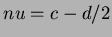
- beta0
- the constant term of the quadratic trend.
- beta1
- a column vector of coefficients of the linear terms. The
vector must be -dimensional.
- beta2
- a matrix of coefficients of the quadratic terms. The
matrix is
 .
.
- x0
- a -dimensional column vector. It indicates the center of
the quadratic trend.
Thus, the quadratic term is of the form:

where is the column vector of variables.
- alpha, theta, sigma2
- They are the
parameters of the covariance function. The default covariance function
we used was
where the default  is the Gaussian isotropic correlation function
Users can select other correlation functions, but we recommend
becoming comfortable with the defaults before doing so. See
Section 3.4.1 for details.
- lower
- the -dimensional vector of lower bounds of the
rectangular design space.
- upper
- the -dimensional vector of upper bounds.
Notice that the krigifier is designed to work in rectangular spaces. If the desired space
is not rectangular, we suggest choosing lower and upper bounds to form a rectangular space that
encloses the desired volume. This may place some design sites outside the desired volume,
but will still result in a random function defined where it is needed.
To create a kriging approximationm, you will need several inputs
- Matrix<double> Points
- This is the matrix of points. These are
your locations.
- Vector<double> Values
- These are the corresponding function values . Thus
![$f(Points[i, \cdot]) = Values[i]$](img62.png) .
.
- int choice
- The choice of correlation function. Defaults to
1. See 3.4.1 for more details on the functions available
- double theta[]
- An array of numbers. This depends on the choice
of correlation function. Generally, the array should contain all the
values of , followed by all the values of . There can be
either 1 or p values
 and 1 or p values of
  .
.
3.9.3 RBF Approximation Parameters
To create a rbf approximation, you will need several parameters.
- Matrix<double> Points
- This is the matrix of points. These are
your locations.
- Vector<double> Values
- These are the corresponding function values . Thus
.
- long deg
- This is the degree of the polynomial basis. If you set
 , it
will use no basis. Then
, it
will use no basis. Then  uses only a constant term. Finally
 uses
uses  number of first degree monomials and a constant term. We recommend choosing
 .
.
- int choice
- The flag for which radial basis function to use. This should be an
integer between 0 and 7. See section 3.4.3
- double c, beta
- These are the parameters for the radial basis function. Not every
basis function needs both, but values should always be passed in.
The krigifier and kriging approximations can provide you with
derivatives of the function at a specified point. The function call
is much like a call to evalf. The function returns the vector
gradient of the function at the point given.
Vector<double> evalderiv( const Vector<double>& point);
In the kriging approximation, this is the derivative of
the approximation function, not an approximation of the
derivative of the original function. While for large enough sample, these derivatives
should be close, for small data sets, there is no guarantee that the values are anywhere
close, and thus this function is not a substitute for derivative information about
the original function.
Note however that while derivatives have been implemented for all
choices of correlation function, we are still testing the
implementations. Correlation functions 1,2,and 3 are known to work.
These are the Gaussian Isotropic, Gaussian Product, and Product Linear
Correlation functions. The other ones are still being tested, so use
them at your own risk. Further, notice that several correlation
functions are not differentiable everywhere. For example, if you choose  then the Gaussian correlation functions are not differentiable at
the interpolated points.
The derivative functions handle taking the derivative of the trend as
well, and adding it in appropriately. Howeve, when using a
user-defined trend, the derivative function will only return
the derivative of the kriging. You must add the derivative of the
user-defined trend to this value in order to get the derivative of the
function. This is because
then the Gaussian correlation functions are not differentiable at
the interpolated points.
The derivative functions handle taking the derivative of the trend as
well, and adding it in appropriately. Howeve, when using a
user-defined trend, the derivative function will only return
the derivative of the kriging. You must add the derivative of the
user-defined trend to this value in order to get the derivative of the
function. This is because
implies that
- 1
-
W. R. Madych and S.A. Nelson.
Multivariate interpolation and conditionally positive definite
functions ii.
Mathematics of Computation, 54(189):211-230, 1990.
- 2
-
Anthony D. Padula.
Interpolation and pseudorandom function generation.
Honors Thesis, Department of Mathematics, College of William & Mary,
Williamsburg, Virginia 23187-8795, May 2000.
- 3
-
Christopher M. Siefert.
Model-assisted pattern search.
Honors Thesis, Department of Computer Science, College of William &
Mary, Williamsburg, Virginia 23187-8795, May 2000.
- 4
-
Michael W Trosset.
The krigifier: A procedure for generating pseudorandom nonlinear
objective functions for computational experimentation.
Interim Report 35, ICASE, 1999.
Documentation for the Krigifier, Kriging Approximation, and Radial Basis Function
Approximation C++ Classes
This document was generated using the
LaTeX2HTML translator Version 99.2beta6 (1.42)
Copyright © 1993, 1994, 1995, 1996,
Nikos Drakos,
Computer Based Learning Unit, University of Leeds.
Copyright © 1997, 1998, 1999,
Ross Moore,
Mathematics Department, Macquarie University, Sydney.
The command line arguments were:
latex2html -split 0 -no_navigation -show_section_numbers documentation.tex
The translation was initiated by Anthony D. Padula on 2000-07-19
Anthony D. Padula
2000-07-19
