-
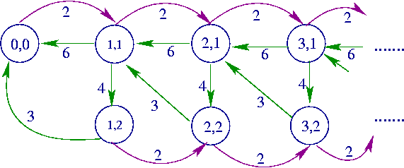
The above Markov chain is countinous time and the
input of the C++ version of the tool should consist of matrixes that define its infinitesimal
generator. The order of the input matrices is showed in the following. Note
that the matrices in this example are simple scalars (the explanations on
the right should not be included in the input file).
| 1 |
Size of
boundary portion |
| 1 |
Size of
repetitive portion |
| 1 |
Burst
size of the process |
| 0.000000000000001 |
Numerical accuracy |
| -2.0 |
Local transitions in boundary
portion |
| 3.0 |
Backward transitions to boundary
portion |
| 2.0 |
Forward transitions from boundary
portion |
| 3.0 |
Backward transitions in the
repetitive portion |
| -5.0 |
Local transitions in the repetitive
portion |
| 2.0 |
Forward transitions in the repetitive
portion |
 > load QBDtestcase1
> G = QBD_G_ETAQA(A);
> pe = QBD_pi_ETAQA(B,A,B0,G);
> meanqlen = QBD_qlen_ETAQA(B,A,B0,pe,1);

-
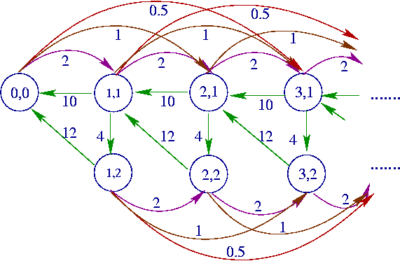
The above Markov chain is countinous time and the
input of the C++ version of the tool should consist of matrixes that define its infinitesimal
generator. The order of the input matrices is showed in the following. Note
that the matrices in this example are simple scalars (the explanations on
the right should not be included in the input file).
| 1 |
Size
of boundary portion |
| 2 |
Size
of repetitive portion |
| 1 |
Burst
size of the process |
| 0.000000000000001 |
Numerical accuracy |
| -2.0 |
Local transitions in boundary
portion |
| 6.0 3.0 |
Backward transitions to boundary
portion |
| 2.0 0.0 |
Forward transitions from boundary
portion |
| 6.0 0.0 3.0 0.0 |
Backward transitions in the
repetitive portion |
| -12.0 4.0 0.0 -5.0 |
Local transitions in the repetitive
portion |
| 2.0 0.0 0.0 2.0 |
Forward transitions in the
repetitive portion |

